
-
- Products
- Indoor Household Cords
- Appliance Cords
- General Purpose Short-Length Cords
- General Purpose Extension Cords
- Landscape & Decorating Cords
- Bright Color Extension Cords
- Oil-Resistant Extension Cords
- Cold-Flex Extension Cords
- VividFlex Power Cords
- EXTREME All-Weather Cords
- Cord Management
- Task Lights
- Adapters & GFCI Devices
- Where to Buy
- About
- Careers
- Glossary
- Catalog


What Is Ultra Wideband Positioning and How Does It Work?
Ultra Wideband Positioning is a precise wireless method for locating people, tools, and equipment indoors. It uses extremely short radio pulses to measure distance between a small tag and fixed anchors. These measurements can produce location data within a few centimeters in suitable conditions. GPS often struggles inside buildings. UWB can continue working where concrete walls block satellite signals.
The process depends on timing. A tag sends a pulse, and anchors record when it arrives. The system calculates distance from the signal’s travel time. Some networks use two-way ranging, while others compare arrival times across multiple anchors. Software then combines these distances to estimate the tag’s position. A worker might carry a badge, while anchors sit near doorways, ceilings, or production lines. The resulting map can show movement through a warehouse almost in real time.
Accuracy is not automatic. Metal shelves, moving bodies, poor anchor placement, and clock errors can distort results. Calibration matters. So does thoughtful installation. Modern UWB solutions may use security features associated with IEEE 802.15.4z, but implementation quality still varies. Privacy also requires careful decisions about data retention and user consent. This technology is powerful, yet it is not magic. A few centimeters in a laboratory may become tens of centimeters on a crowded factory floor. This guide explains how Ultra Wideband Positioning works, where it performs well, and why practical testing remains essential. Some assumptions may fail in unfamiliar buildings. That is worth remembering.
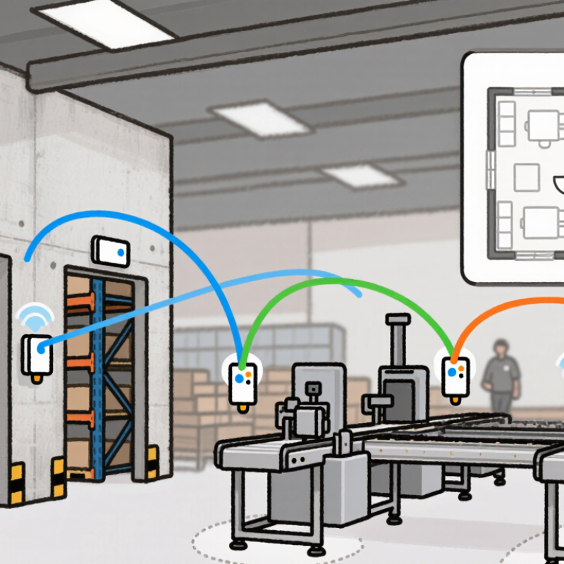
Table of Contents [Hide]
What Ultra-Wideband Positioning Means
Ultra-wideband positioning means locating objects or people through very short radio pulses. Unlike systems that estimate distance from signal strength, UWB measures how long a pulse takes to travel. The result can be accurate to roughly tens of centimeters in suitable conditions. That sounds simple, but real spaces are rarely simple.
A positioning system usually includes fixed anchors and mobile tags. Anchors sit around a room, while a tag sends signals between them. The system calculates distance from signal travel time, then combines several measurements to estimate location. Walls, metal surfaces, crowded rooms, and poor anchor placement can reduce accuracy. Reflected signals may also create unstable readings. Calibration matters more than many quick demonstrations suggest. Even then, small errors remain.
Tips: Place anchors at different heights and keep them away from large metal objects. Test accuracy while people move through the space. Record errors, not only successful results. Use UWB for clear location data, but avoid treating every measurement as perfect. A backup sensor can improve reliability when signals become blocked.